None
[2]:
import numpy as np
Author: Pierre Ablin
Integrating mvlearn with scikit-learn
mvlearn mimics most of scikit-learn API, and integrates seamlessly with it. In scikit-learn, a dataset is represented as a 2d array X of shape (n_samples, n_features). In mvlearn, datasets Xs are lists of views, which are themselves 2d arrays of shape (n_samples, n_features_i). The number of features does not have to be constant:
[3]:
n_samples = 100
n_features1 = 20
n_features2 = 30

X1 = np.random.randn(n_samples, n_features1)
X2 = np.random.randn(n_samples, n_features2)
Xs = [X1, X2]
Here, Xs is a multiview dataset, containing two views. mvlearn works with these objects.
ViewTransformer
mvlearn.preprocessing.ViewTransformer is a handy tool to apply the same sklearn transformer to each view of the multiview dataset. For instance, it is simple to apply PCA to each view. In the following, we reduce the dimension of each view to 3:
[4]:
from mvlearn.preprocessing import ViewTransformer
from sklearn.decomposition import PCA

pca = PCA(n_components=3)
mvpca = ViewTransformer(pca)
Xs_transformed = mvpca.fit_transform(Xs)
print(len(Xs_transformed))
print([X.shape for X in Xs_transformed])
2
[(100, 3), (100, 3)]
The PCA is applied to each view with the mvpca transformer, and the output of PCA, Xs_transformed, is a multiview dataset, where each view now has 3features.
Importantly, it is possible to apply a different transform to each view, by passing a list to ViewTransformer. For instance, if we want to keep 5 components in the second dataset, we can do:
[5]:
pca2 = PCA(n_components=5)
mvpca = ViewTransformer([pca, pca2])
Xs_transformed = mvpca.fit_transform(Xs)
print(len(Xs_transformed))
print([X.shape for X in Xs_transformed])
2
[(100, 3), (100, 5)]
Mergers
At the end of a multiview machine learning pipeline, it is sometimes needed to transform the multiview dataset in a single view dataset. All sklearn methods can then be used on this single view dataset. Mergers make this task simple.
A simple way to transform a multiview dataset in a single view dataset is simply by stacking each features. The class mvlearn.compose.ConcatMerger implements this:
[6]:
from mvlearn.compose import ConcatMerger

merge = ConcatMerger()

X_transformed = merge.fit_transform(Xs)
print(X_transformed.shape)
(100, 50)
This allows for simple integration in scikit-learn pipelines.
Pipeline example: group-ICA
As a simple illustration, we now show how easy it is to code group independent component analysis (groupICA) from scratch using mvlearn.
We use the group ICA of Calhoun et al. “A method for making group inferences from functional MRI data using independent component analysis.”, Human brain mapping 14.3 (2001): 140-151. as reference.
GroupICA takes a multiview dataset, and tries to extract from it some shared independent sources. In its usual formulation, it consists of three simple steps:
- Apply an individual PCA to each view
- Concatenate the features of each view
- Apply usual ICA on the concatenated features
This is easily implemented using mvlearn and scikit-learn pipelines:
[7]:
from sklearn.decomposition import FastICA
from sklearn.pipeline import Pipeline

n_components = 2
individual_pca = ViewTransformer(PCA(n_components=n_components))
merge = ConcatMerger()
ica = FastICA(n_components=n_components)

groupica = Pipeline([('individual pca', individual_pca),
                     ('concatenate', merge),
                     ('ica', ica)])

X_transformed = groupica.fit_transform(Xs)
print(X_transformed.shape)
(100, 2)
Here, Xs contains Gaussian noise, so nothing of value is extracted. However, if each view consists of a linear transform of some independent sources, it works as intended:
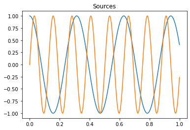
[8]:
import matplotlib.pyplot as plt
time = np.linspace(0, 1, 1000)
source1 = np.cos(20 * time)
source2 = np.sin(50 * time)
S = np.c_[source1, source2]
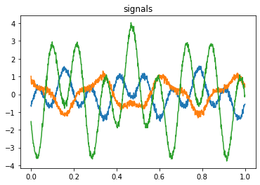
A1 = np.random.randn(3, 2)
A2 = np.random.randn(4, 2)
X1 = np.dot(S, A1.T) + .1 * np.random.randn(1000, 3)
X2 = np.dot(S, A2.T) + .1 * np.random.randn(1000, 4)
Xs = [X1, X2]
plt.figure()
plt.plot(time, source1, time, source2)
plt.title('Sources')
plt.figure()
for x in X1.T:
plt.plot(time, x)
plt.title('signals');
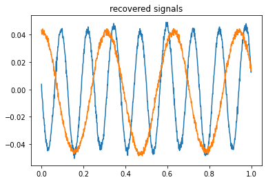
[9]:
X_transformed = groupica.fit_transform(Xs)
[10]:
for x in X_transformed.T:
    plt.plot(time, x)
plt.title('recovered signals');